This page provides a simplified description of the orbital mechanics that determine the solar radiation throughout the year and day. Knowing the date, local time, latitude and longitude, an estimate of the solar radiation can be calculated. Knowing the size, orientation and efficiency of the solar panels, and the efficiency of the converter used to charge the battery system, the power available to charge the battery can be calculated. Finally, knowing the load power lets us simulate the energy flow over a multiple day period to see how well the system will perform and whether more or less panels, battery capacity, etc. is required.
Declination and the Seasons
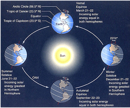
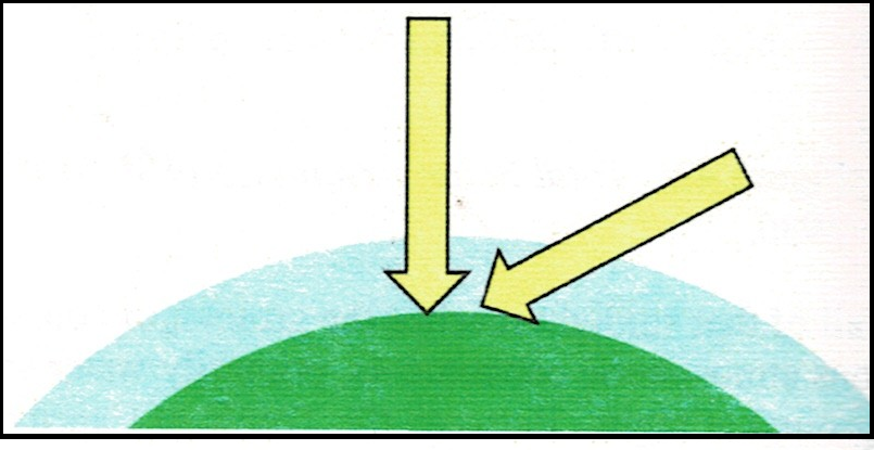
The Earth orbits the sun in a nearly circular orbit in a plane known as the ecliptic once per year. It also rotates about a North-South axis once per day. The plane normal to the North-South axis that passes through the center of the Earth is the equatorial plane. These two planes, the ecliptic and equatorial are not the same. As shown in the above figure, the North pole tilts toward the sun around the summer solstice and away from the sun around the winter solstice. The Northern hemisphere then get more solar energy around the summer solstice and the Southern hemisphere less. This explains why we have seasons and why they are reversed in the Northern and Southern hemispheres.
The tilt between the North-South axis and the normal to the ecliptic is 23.45 degrees. An observer at the equator would see the angle between the equatorial plane (the local vertical axis) and the sun at its highest point in the day vary throughout the year from +23.45 degrees (North) at summer solstice to -23.45 degrees (South) at winter solstice. This angle δ is known as the declination angle of the sun.
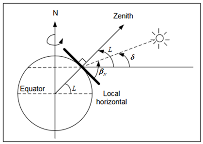
At other locations on the Earth, the local vertical relative to the equatorial plane is equal to the latitude L as shown above. The sun angle at solar noon βN is measured from the local horizontal to the sun angle. The declination however is measured from the equatorial plane to the sun angle so it does not vary with location. So now we have two useful equations:
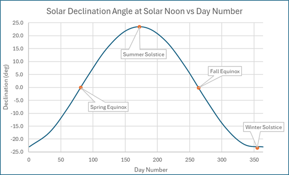
δ = 23.45 sin[(360/365)(n – 81)]
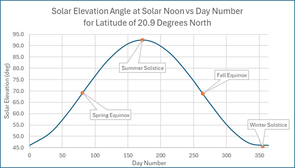
βN = 90° – L + δ
The new variable n is the day number. It starts with n = 1 on January 1. Some other important days are listed below. The sun angle depends on the latitude, so the values shown below are based on this year at my location in San Miguel de Allende, Mexico which has a latitude L of +20.9 degrees.
| Name | n | Date | δ | βN (SMA) |
| Spring Equinox | 81 | 3/22/2025 | 0.0 | 69.1 |
| Summer Solstice | 172 | 6/21/2025 | 23.45 | 92.5 |
| Fall Equinox | 264 | 9/21/2025 | -0.2 | 68.9 |
| Winter Solstice | 355 | 12/21/2025 | -23.45 | 45.7 |
The graphs below show the variation of the declination angle and the solar elevation at solar noon.
Beam Irradiance
The solar irradiance is a measure of the intensity of the radiation from the sun. Beam irradiance IB indicates that the radiation is at right angles to the plane or panel receiving the radiation. It is measured in watts per square meter.
The solar beam irradiance is reduced from that outside the atmosphere by the absorption of energy passing through the air. Since it must pass through much more air mass near sunset or sundown, the beam irradiance is much lower at these times then at solar noon.
The beam irradiance can be calculated from the following equations:
IB = 1353∙0.7AM^0.678
AM = 1/cos(β)
AM is called the air mass ratio and β is the sun elevation angle.
The next section discusses the calculation of both solar azimuth and elevation during the day of the year and hour of the day. Using those results, the beam irradiance can be calculated for any location vs local time for any day of the year.
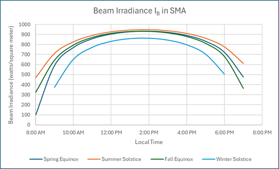
Note that the beam irradiance is fairly constant for the 5 or so hours centered on solar noon. But remember this is the intensity delivered to a flat surface at right angles to the beam. It would require a tracking system to collect this energy.
Obliquity
If a flat surface of one square meters in area is placed at right angles to the sun line it would see the beam intensity discussed above. But if it is at any other angle, the intensity would be reduced as it is spread out over a larger area that is not collected by the one square meter surface.
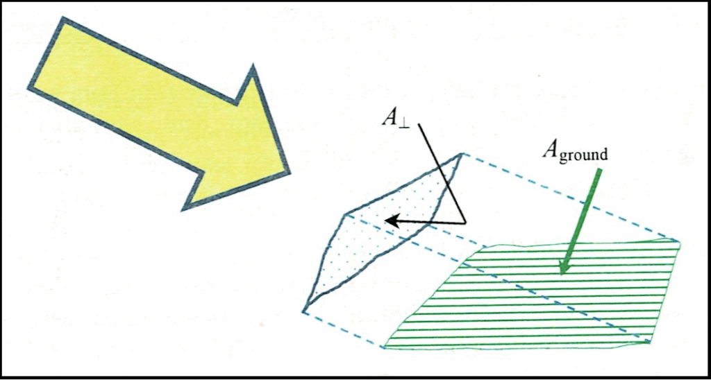
To calculate the effect of the obliquity between a solar panel and the sun angle consider the following figure.
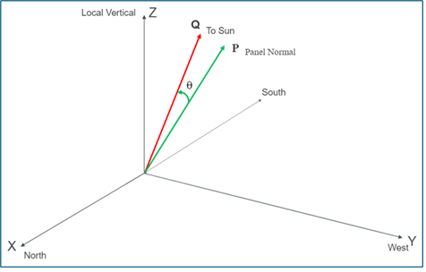
Q is a line directed at the sun from the center of the solar panel and P is a line normal to the panel. The two lines may be misaligned in both the North-South and East-West directions. The angle θ is the angle between them. The irradiance on the collector (solar panel) IBC is
IBC = IB cos(θ)
Getting the angle θ is a bit complicated because of the way the sun angle and panel angles are specified.
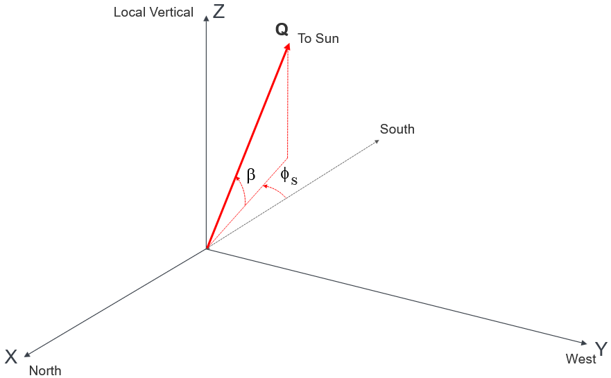
The sun elevation angle β is measured from the local horizontal plane to the sun line and the sun azimuth angle φS is defined as positive counterclockwise from the South direction. This is different from the usual definition of azimuth (positive clockwise from North).
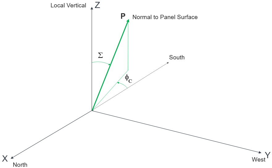
The direction of the normal to the solar panel P is similarly defined by an azimuth φC positive counterclockwise from South and a tilt angle Σ measured down from the local vertical.
The peculiar choice of these coordinates makes the math messy, but the final result is
cos(θ) = cos(β)cos(φS – φC)sin(Σ) + sin(β)cos(Σ)
If, as is usually done, the solar panel is aimed South and tilted to the angle corresponding to the latitude, things simplify as φC = 0 and Σ = L. Then,
cos(θ) = cos(β)cos(φS)sin(L) + sin(β)cos(L)
The sun angles β and φS vary with the day of the year and time of day. These calculations get ugly, but fortunately, there are some really good calculators available to do this. The most convenient one is the NOAA Solar Calculations Day Excel spreadsheet that can be downloaded from https://gml.noaa.gov/grad/solcalc/NOAA_Solar_Calculations_day.xls
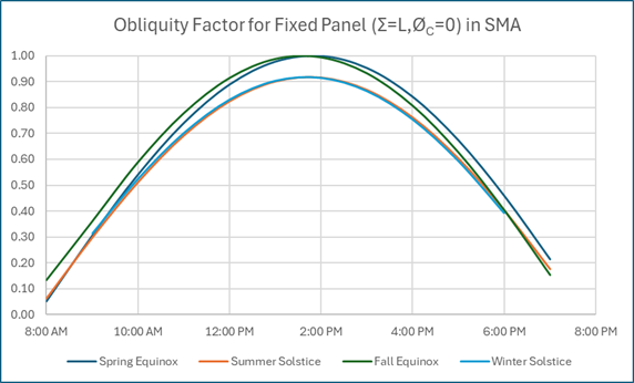
As an example, the obliquity factor, IBC/IB = cos(θ), was calculated for a solar panel aimed South and tilted to the latitude 20.9 degrees for San Miguel de Allende.
Efficiency, Cloud Cover and Panel Area
There are several other factors to consider, then we can combine all of this into a prediction of the charging power of the solar panel system for any day or time.
All of the calculations to this point assumed a clear sky. However cloud cover will reduce the radiant power by the factor 0.75(1-F3) where F is the percentage cloud cover. For a 100% cloudy sky, 25% passes through. For 25% cloud cover, 74% gets through. The latter seems a reasonable assumption for my location.
IBC = 0.74 IB cos(θ)
The solar panels themselves have a rated efficiency in converting solar power into DC electrical power output. The panels I used (Luxen Solar LNET-660M) have an active area of 3.11 square meters each and an efficiency of 20%. Three panels are used so total surface area is 9.33 square meters.
Ppanel = IBC (9.33)(0.2) watts
The generator (converter) has an efficiency less than 100% in converting the DC panel power or energy into the energy stored in the battery system then into the AC energy delivered to the load. There is also a limit on the solar input charging power. For the Ecoflow Delta Pro Ultra I selected, the upper limit on the low voltage panel input is 1.6 kW. There is no specification on the efficiency but some customers have measured it at about 75%.
Pcharge = MIN(.75 Ppanel , 1600)
At this point, you may be thoroughly confused as to where all this is headed. The following chart attempts to make it clear as to what parameters are needed to make the various steps needed to calculate the charging power.
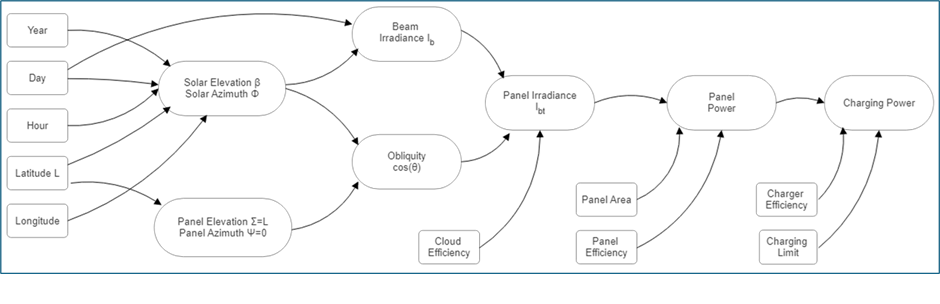
Putting this all together, the charging power was calculated for my system in San Miguel assuming 25% cloud cover, 3 LNET-660M panels oriented South, tilted 21 deg, etc.
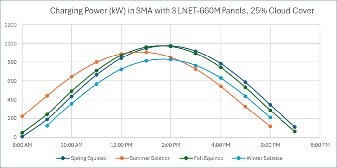
The cumulative energy of this system for each of the following days is:
| Day | Energy (kWh) |
| Spring Equinox | 6814 |
| Summer Solstice | 6507 |
| Fall Equinox | 6819 |
| Winter Solstice | 5460 |
Simulated Performance Under Load
We can now see how this system would work under various load condition. The worst case is during Winter Solstice, so we can use that as the charging power and integrate to get the cumulative battery energy. The battery is restricted to 6.0 kWh so we need to see if that is exceeded. The load will vary throughout the day, but it averages 0.25 kW, so we can use that as a constant. The worst case starting condition is with the battery fully discharged at midnight when the simulation begins.
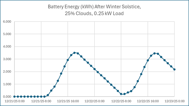
In this plot, each dot corresponds to one hour and the simulation runs for two days. Since there is no sun and no initial charge, the stored energy in the battery remains at zero from midnight until sunrise around 9:00. The battery charges slowly with no load power being delivered until about noon when the 250 watt load can be supplied. At the end of the first day, the total energy supplied to the load is 3.25 kWh and the total energy supplied to the battery by the panels is 5.46 kWh. At this point, the battery is holding 2.21 kWh.
Unlike the first day, the battery supplies load throughout the second day. During day two, the total energy supplied to the load is 5.50 kWh, the energy supplied by the panels is again 5.46 kWh and the battery ends up holding 2.17 kWh.
References
Energy A Textbook, Howard C. Hayden
Renewable and Efficient Electric Power Systems, Gilbert M. Masters
Thermal Environmental Engineering, James L. Threlkeld
“Photovoltaics Education Website,” www.pveducation.org, C.B.Honsberg and S.G.Bowden